Part 1: Introduction to Probability
Chapter 1: Bayesian thinking and everyday reasoning
The central theme of this chapter: Data informs beliefs; belief should not inform data Let’s consider two world views in regard to data:
- (Ideal framework): “the probability of data given my hypothesis and experience in the world” or “how well do my beliefs explain the world?”
- (not ideal): “the probability of my beliefs given the data and my experience in the world” or “how well what I observe supports what I believe”
The first case is where we change our beliefs according ot he data
The second case gathers data (cherry picking) to support our existing belief
Bayesian thinking is about changing your mind and updating how you understand the world until your new beliefs align with the data.
Chapter 2: Measuring uncertainty of binary outcomes
You can calculate the odds that your hypothesis is more probable than your counterpart’s hypothesis by waging bets and calculating the ratio between the two. This assumes:
- The outcome is binary
- The probabilities are uncertain, so we proxy the probabilities by our confidence in how much we’re willing to bet.
Chapter 3: The logic of uncertainty
In this chapter, we review the product rule and sum rule for independent and mutually excuse events.
To recap:
-
Independent: the outcome of one event does not impact the outcome of the next event
-
Mutually exclusive: An event cannot happen at the same time as another event
-
(independent and mutually exclusive): rolling a 6 is mutually exclusive and independent of rolling a 2
-
(independent but not mutually exclusive): a basketball game being canceled because the coach is sick is independent of the game being canceled due to weather; but the coach being sick and rain occurring are not mutually exclusive
-
(dependent and mutually exclusive): weather forecast between a sunny day and a rainy day; if it’s raining, then the probability of it being sunny is affected. Furthermore, it cannot rain at the same time we have clear skies, so the two events are mutually exclusive
-
(dependent and not mutually exclusive): “rolling an even number” and “rolling a number greater than 4.”
Chapter 4: Creating a binomial probability distribution
A review of when to use binomial formula:
- Binary outcome
- Fixed number of trials
- Constant probability of success throughout the trials
- Independence between trials
If these conditions are met, then we may use the binomial formula to answer questions like:
- What is the probability of getting exactly k successes?
- What is the probability of getting at least k successes?
- What is the probability of getting at most k successes?
- What is the probability of getting between x and y successes (inclusive)?
- What is the probability of getting no successes?
The formula for binomial probability is:
P(X = k) = C(n, k) * p^k * q^(n-k)
Where:
- P(X = k) is the probability of getting exactly k successes.
- n is the total number of trials.
- k is the desired number of successes.
- p is the probability of success on a single trial.
- q is the probability of failure on a single trial (q = 1 - p).
- C(n, k) represents the binomial coefficient, which is calculated as n! / (k! * (n - k)!)
Chapter 5: The Beta Distribution
In real life we are almost never sure what the exact probability of any event is; instead, we just have observations and data.
This is the statement that separates statistics from probability.
In probability, we know exactly how probable events are. In statistics, we look at the problem in reverse, and the task of figuring out probabilities given data is called inference.
The binomial formula works well only when we know the probability of success, p., but what do we do when we’re not certain what that probability is?
That’s exactly where the beta distribution comes in. The beta distribution gives us the ability to determine the probability of a collection of probabilities
The beta distribution helps us determine the probability of a collection (distribution) of probabilities that could represent the true value of p (probability of success) in a binomial distribution
The true value of p is one that we can infer to be the most probable from the beta distribution
Part 2: Bayesian probability and prior probabilities
Chapter 6: Conditional probability
Part 1 was all about independence events where the outcome of one trial does not influence the outcome of the next trial.
As we ascend to more complex issues, we start discovering that certain events depend on others.
Bayes theorem allows us to take our belief about the world, combine them with data, and then transform this combination into an estimate of the strength of our beliefs given the evidence we have observed
Chapter 7: Bayes’ theorem with lego
A review of Bayes’ theorem
Chapter 8: The prior, likelihood, and posterior of bayes theorem
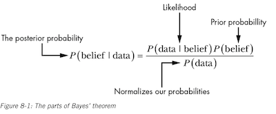
The goal of Bayes Theorem is to quantify how strongly we hold our beliefs given the data we’ve observed (the posterior probability, P(belief | data)).
The likelihood is the probability of the data to exist given our belief (P(data | belief)).
Finally, the prior probability tells us the plain-jane probability of our data to exist by itself (P(belief))–this represents the strength in our belief before seeing any data.
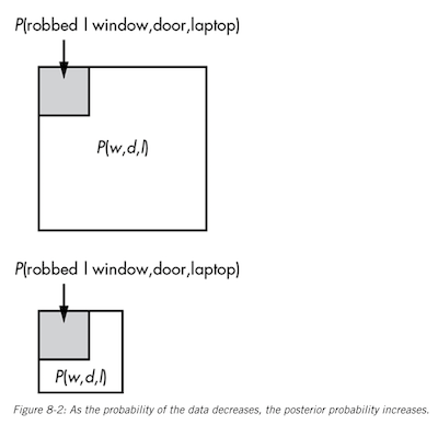
Since the probability of the data is in the denominator, this means that as the probability of the data increases, the probability of our posterior decreases, because as the data we observe becomes increasingly unlikely, a typically unlikely explanation does a better job of explaining the event.
Chapter 9: Bayesian Priors and working with probability distributions
Prior probabilities are the most controversial aspect of Bayes’ Theorem because they’re frequently considered subjective.
Part 3: Parameter Estimation
Chapter 10: Introduction to Averaging and Parameter Estimation
Parameter estimation is a statistical inference technique where we use our data to guess the value of an unknown variable.
Taking the average of a measurement is a good start at inference. Averaging data is useful because there’s an equal probability of our estimate being higher or lower to some degree from the true value. In other words, errors in measurement tend to cancel each other out.
Chapter 11: Measuring the spread of our data
In this chapter, we learn about standard variance and variance for quantifying the spread of our data.
Chapter 12: The Normal Distribution
A review of the normal distribution
Chapter 13: Tools of Parameter Estimation: PDF, CDF, and Quantile
Helpful in determining the confidence interval of our given estimation.
Chapter 14: Parameter Estimation with Prior Probabilities
This is where we use out existing beliefs to get a parameter estimation, or how the beta distribution changes as we gain more info.
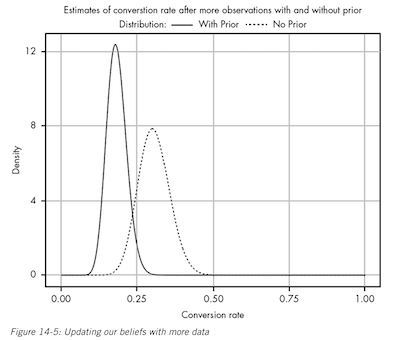
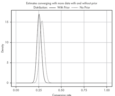
The more data we gather, the more our prior beliefs become diminished by evidence. But before that, in light of new evidence, our prior beliefs squashed any data we had. A prior probability can help keep our estimate more accurate in the absence of data.
The best priors are backed by data, and there is never really a “fair” prior when you have a total lack of data. Everyone brings to a problem their own experiences and perspectives on the world.
The value of Bayesian reasoning, even when you are subjectively assigning priors, is that you are quantifying your subjective belief; this permits you to compare your prior with other people’s and see how well it explains the world around you.
Likewise, no amount of mathematics can make up for ignorance. If you have no data and no prior understanding of the problem, the only honest answer is to say that you can’t conclude anything until you know more.
Part 4: Hypothesis Testing: The heart of statistics
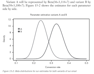
Chapter 15: From parameter estimation to hypothesis testing: building a bayesian A/B test
Bayesian A/B test can work well when testing two cases.
If we are checking click rates on email subscriptions, and we already have an idea, either from industry knowledge or past data, of the click rate probability, then that can serve as our prior.
Then, the A/B testing can be performed to give us the likelihood. And, once we have the likelihood, we can combine the prior and likelihood to get our posterior distribution.
But how sure can we be that version B is better than version A? That’s where Monte Carlo simulations come into play.
We can imagine the posterior distribution to represent all the worlds that could exist based on our current state of beliefs from the data.
Every time we sample from each distribution we’re seeing what one possible world could look like.
We can tell from from the above figure to expect more worlds where B is the truly better variant, and the more frequently we sample, the more precisely we can tell in exactly how many worlds, of all the worlds we’ve sampled, B is the better variant. This is fundamentally the Monte Carlo method.
Once we have our samples, we can look at the ratio of worlds where B is the best to the total number of worlds sampled, thereby giving us an exact probability that B is in fact greater than A.
Note: the remainder of this chapter has a great walk through of running the sampling and the beta distributions in R. Review this chapter if you seek implementation.
Chapter 16: Introduction to the Bayes Factor and Posterior odds: The competition of ideas
Recall for formula for Bayes’ theorem. The hardest part of the formula for P(H|D) is in calculate the probability of our data P(D).
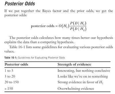
P(D) is also the denominator of our formula, which means that if we are more interested in comparing two hypothesis, rather than computing the actual probability (which includes calculating P(D)), we can instead compute the ratio of posteriors formula.
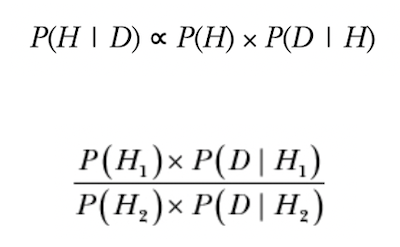
We call the result of this ratio the posterior odds. And, when we factor our P(H) for two hypothesis that are equally likely on their own, we get the Bayes Factor, which is the ratio between the likelihoods of two hypotheses.
In Bayesian reasoning, we’re not gathering evidence to support our ideas; we’re looking to see how well our ideas explain the evidence in front of us.
What the ratio is telling us is the likelihood of what we’ve seen given what we believe to be true, compared to what someone else believes to be true. Our hypothesis wins when it explains the world better than the comparing hypothesis.
But the alternative could be true; it could be the case that the other person’s hypothesis is correct, in which case we may consider changing our own beliefs.
The key here is that in Bayesian reasoning, we don’t worry about supporting our beliefs–we are focused on how well our beliefs support the data we observe. Data can either confirm our belief, or lead us to change our minds.
The remainder of this chapter uses a really cool and easy to follow example of testing our with dice.
It’s important to note that while the bayes factor can provide a useful back-of-the-envelope analysis, it alone can’t be used as a single say–it’s only a means of comparing two hypotheses.
Calculating the posterior odds is a more formula and useful test.
Why the davy would I use Bayes Reasoning when I can use a simple Chi-Square test to see if the dice is fair?
It’s all about the data you have available to you.
A chi-square test would work well if you were only observing the outcome of the dice. But, from the example provided in the book, we also know that there’s a 1 in 3 chance we will get a loaded dice.
The difference lies in how much perspective we have.
Bayes’ theorem provides a framework for incorporating prior knowledge and adjusting probabilities based on new data.
The chi-square test does not involve prior beliefs or probabilities. Instead, it compares observed frequencies to expected frequencies under the null hypothesis of no association or no difference between groups. It provides a measure of how well the observed data fit the expected distribution, allowing you to determine if the deviation is statistically significant.
Chapter 17: Bayesian Reasoning in the Twilight Zone
The purpose of this chapter is to quantify how much data it should take to convince someone of a hypothesis.